Reading the market in 280 characters
A model can score well on financial sentiment and still miss the warnings a risk team cares about. I compared six approaches to see where that happens, and whether a finance-specific language model actually helps.
Financial headlines often look easy to classify. “Upgrade”, “beat” and “record profit” sound bullish. “Downgrade”, “miss” and “loss” sound bearish. A simple model should be able to learn that vocabulary quickly.
The difficulty begins when the same words change meaning with context. Rising oil output may be bearish for crude prices. A “funding squeeze” can appear in a bullish headline if a central bank has just relieved it. Even a technically accurate classifier can be poorly suited to market monitoring if most of its mistakes are missed bearish stories.
I tested five traditional machine-learning models and a FinBERT-based classifier on 3,365 labelled financial tweets. FinBERT produced the best overall result. The more useful finding, however, was how sharply the models differed in the mistakes they made.
The sample was only mildly unbalanced
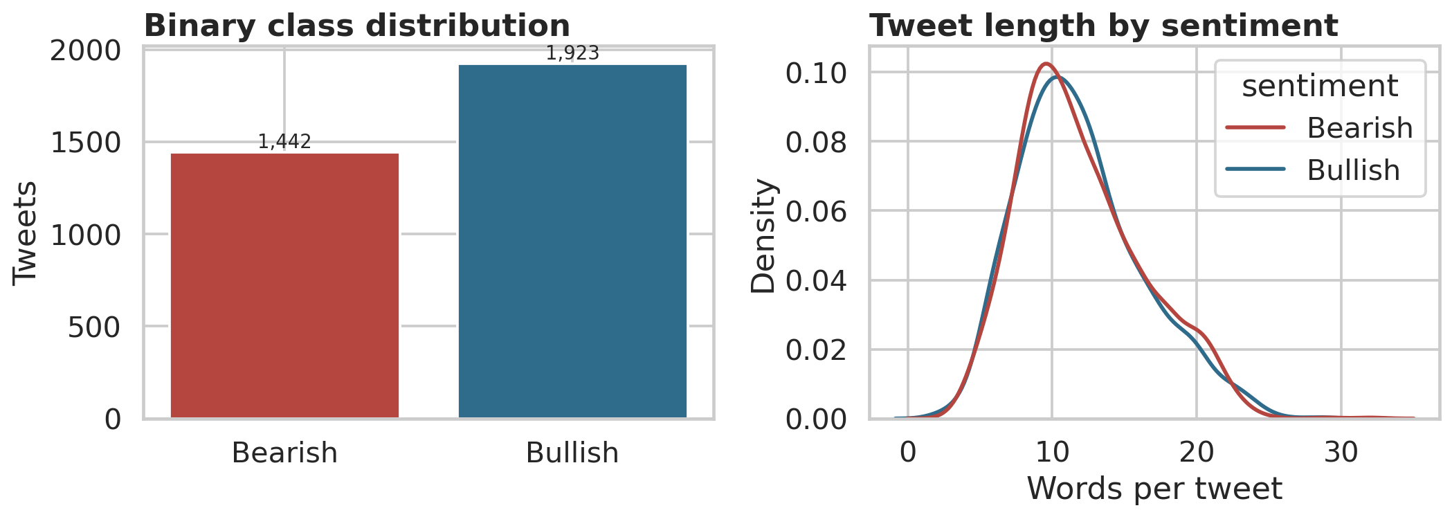
The source data contains 9,543 English-language financial tweets labelled bearish, bullish or neutral. I removed the neutral class for the binary comparison, leaving 1,442 bearish and 1,923 bullish observations.
That 43/57 split is not extreme. It is still enough to reward a model that leans bullish, particularly when performance is judged by accuracy alone. Tweet length offered no easy shortcut: both classes averaged about 12 words.
The reassuring number concealed the important one
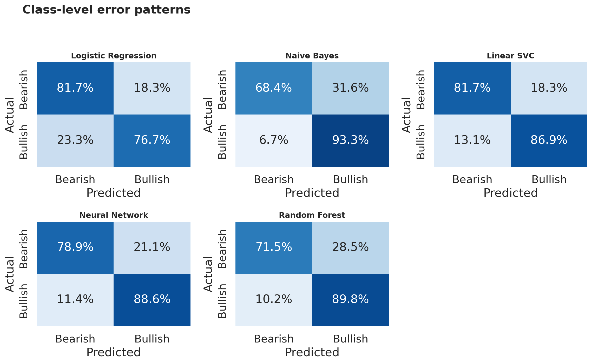
Naive Bayes achieved 82.7% accuracy. Read in isolation, that sounds respectable. Its bearish recall was only 68.4%, meaning that almost one in three bearish tweets passed through as bullish.
The Linear Support Vector Classifier was the strongest traditional model. It reached 84.7% accuracy and detected 81.7% of bearish tweets. A small neural network came close, but its bearish recall was lower. Random Forest also favoured the majority bullish class despite class weighting and grid search.
| Model | Accuracy | Balanced accuracy | Macro-F1 | ROC-AUC | Bearish recall | Bullish recall |
|---|---|---|---|---|---|---|
| FinBERT + Logistic Regression | 87.6% | 87.6% | 87.4% | 0.943 | 87.3% | 87.9% |
| Linear SVC | 84.7% | 84.3% | 84.3% | 0.927 | 81.7% | 86.9% |
| Neural Network | 84.4% | 83.8% | 84.0% | 0.912 | 78.9% | 88.6% |
| Naive Bayes | 82.7% | 80.9% | 81.6% | 0.918 | 68.4% | 93.3% |
| Random Forest | 81.9% | 80.6% | 81.1% | 0.911 | 71.5% | 89.8% |
| Logistic Regression | 78.9% | 79.2% | 78.7% | 0.879 | 81.7% | 76.7% |
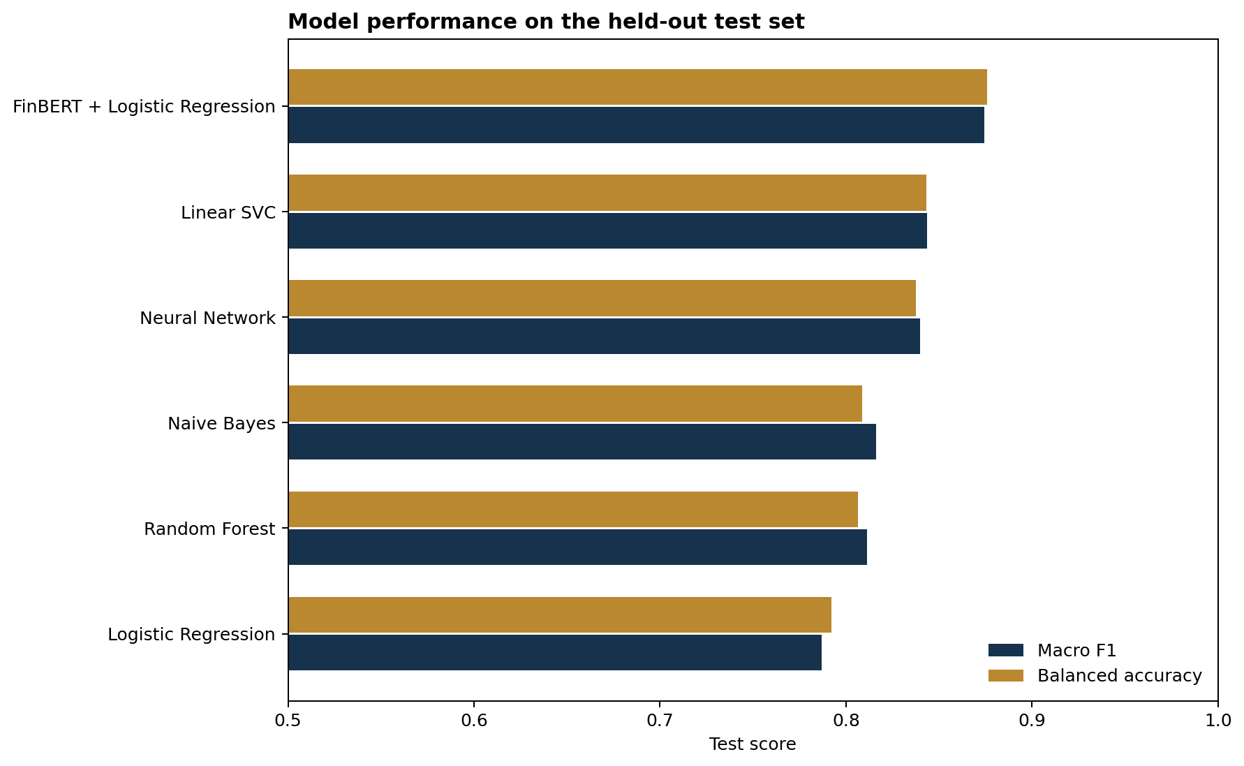
FinBERT improved macro-F1 by 3.1 percentage points over Linear SVC. More importantly, its recall was balanced across the two classes. The model was not simply becoming better at the easier or more common case.
A model can learn the vocabulary without understanding the story
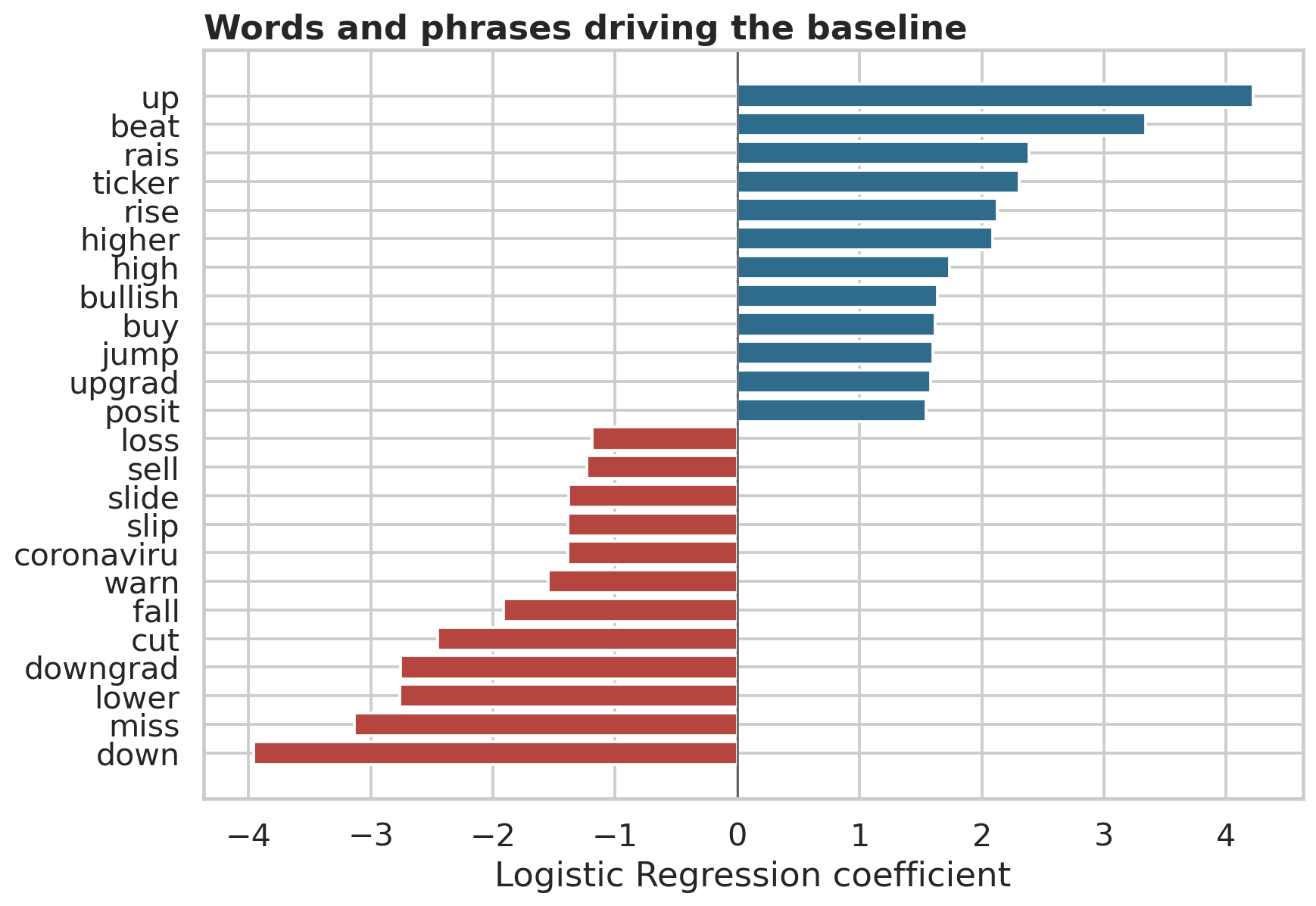
The Logistic Regression coefficients are easy to recognise. “Up”, “beat”, “raise” and “upgrade” pull the model towards bullish. “Down”, “miss”, “lower” and “downgrade” pull it towards bearish. This is useful evidence that the classifier has learned a plausible financial lexicon rather than an arbitrary statistical pattern.
It also exposes a weakness. The generic ticker token carries a positive coefficient, reflecting the way cashtags appear in this particular sample. That relationship may disappear in another period or platform. It should be treated as a data characteristic, not a market rule.
The clearest failures came from headlines where individual words pointed in the wrong direction:
“EIA forecasts U.S. shale oil output to climb…” The model reads “climb” as positive, while higher supply can weigh on oil prices.
“Fed’s ‘bazooka’ soothes dollar funding squeeze.” The alarming vocabulary describes a supportive intervention.
“More stockmarket volatility, less buying the dip, and slower earnings per share growth ahead…” Familiar bullish phrases sit inside an explicitly negative outlook.
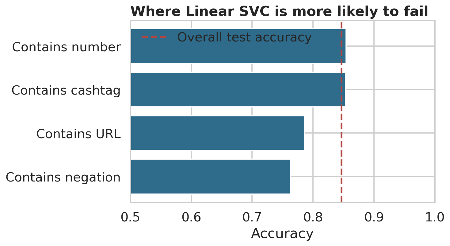
Negation was the weakest identifiable text slice. Linear SVC accuracy fell from 84.7% overall to 76.3% on tweets containing terms such as “not”, “less” or “without”. Link-heavy tweets were also harder because removing the URL sometimes left only a short, ambiguous headline.
Context helped, but it did not make the problem disappear
FinBERT was trained on financial text before it saw this dataset. I used its contextual embeddings as inputs to a balanced Logistic Regression classifier. Unlike TF-IDF, the representation of a word changes with the sentence around it.
The result was the best in the comparison: 87.6% accuracy, 87.4% macro-F1 and 0.943 ROC-AUC. Bearish recall rose to 87.3%. The gain is meaningful, although far from perfect. Labels can depend on the referenced security, the investor’s horizon and information that is not present in the tweet.
A finance-specific language model reduced the imbalance between bullish and bearish errors. It did not remove the need for judgement.
In practice, the threshold matters as much as the model
A market-monitoring team may care more about missing adverse news than reviewing an extra false alert. That changes the decision rule.
I selected a more sensitive Linear SVC threshold using out-of-fold training predictions, targeting at least 90% bearish recall. On the untouched test set, it detected 92.2% of bearish tweets. The price was a higher review burden: 25.8% of bullish tweets were incorrectly flagged, while bearish-alert precision fell to 72.9%.
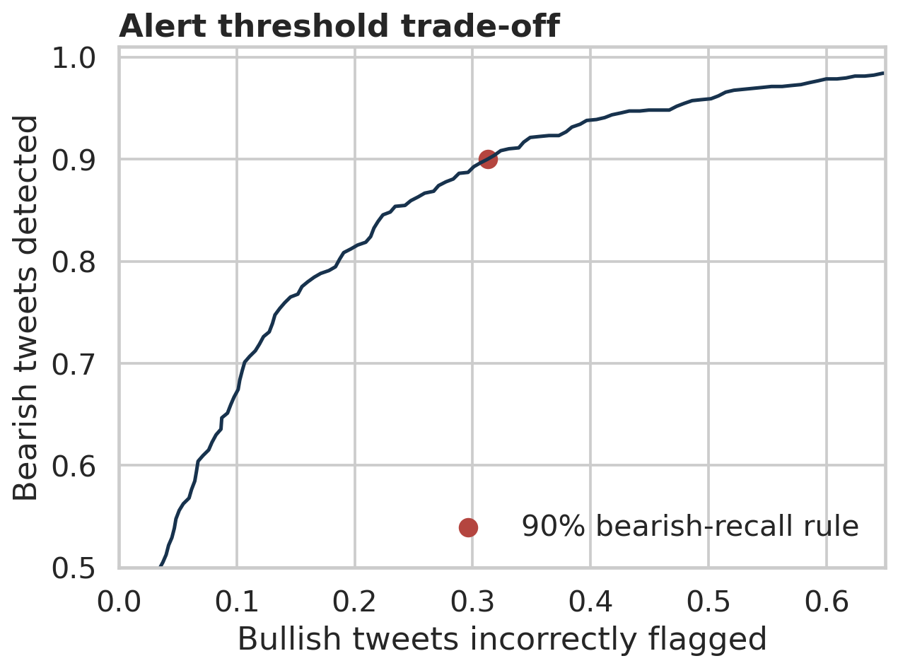
This is a more realistic way to think about deployment. The model would not decide whether to trade. It could rank an incoming news queue, surface potentially adverse headlines and send uncertain cases to an analyst. The threshold would depend on staffing capacity, false-alert costs and the assets being monitored.
A useful workflow would keep the original headline, model score and explanation together. Analysts could correct labels during review, creating the feedback needed to measure drift and retrain the model when vocabulary changes.
What the result does not prove
This is a language-classification result, not evidence of a trading signal. The dataset does not include timestamps, security identifiers, price reactions or transaction costs. A random train/test split cannot measure how performance changes through time.
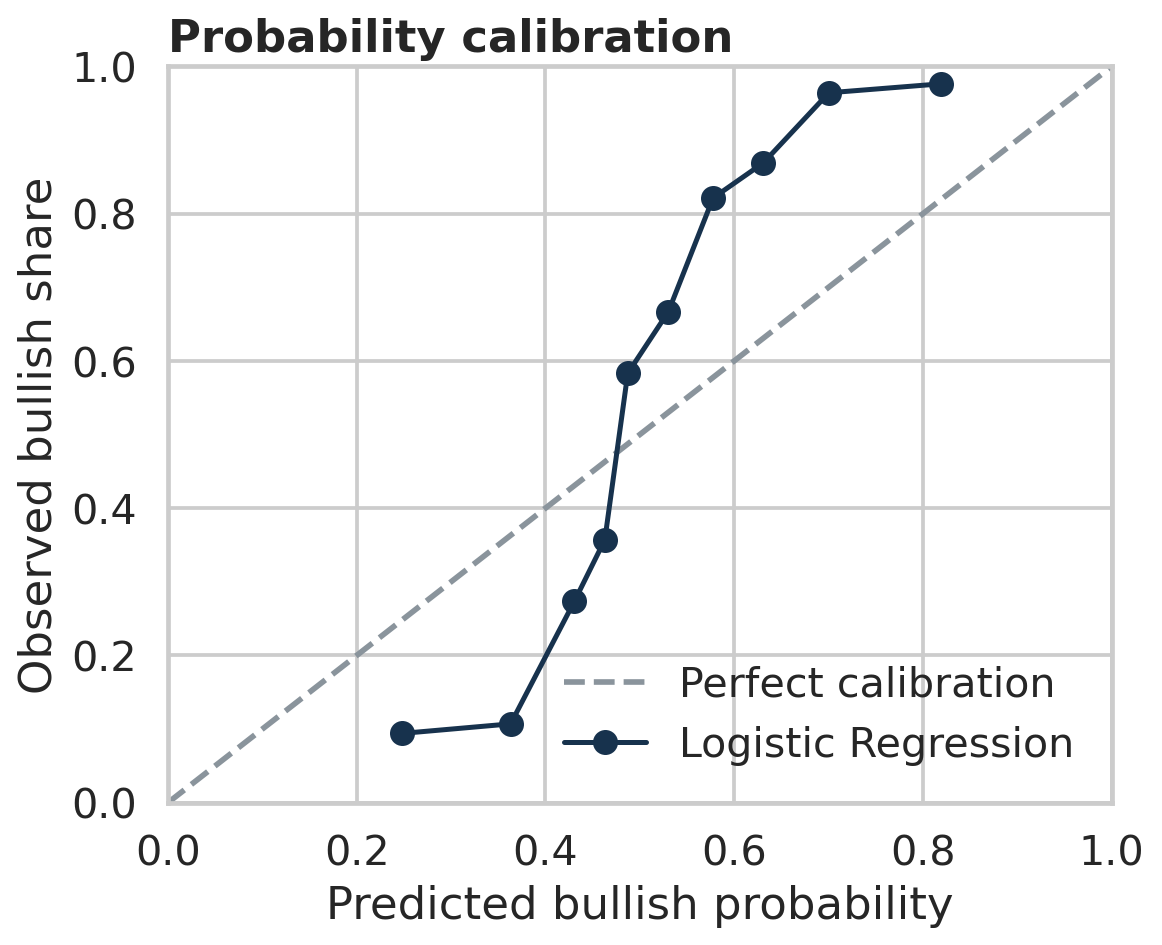
A production test would restore the neutral class, use dated observations and reserve the most recent period for evaluation. It would also measure calibration, latency and drift. Only then could the sentiment score be tested against subsequent returns, volatility or credit-spread changes.
The distinction matters. Classifying a headline correctly and extracting tradable information from it are different problems.
How the comparison was run
Sample
Neutral tweets were removed, leaving 3,365 binary observations. The split contains 2,523 training and 842 test tweets.
Preprocessing
URLs were removed, cashtags were normalised, words were stemmed and TF-IDF used unigrams and bigrams.
Validation
TF-IDF remained inside each five-fold pipeline, preventing vocabulary and document-frequency leakage across validation folds.
Models
The comparison covers Logistic Regression, Naive Bayes, Linear SVC, a two-layer neural network, tuned Random Forest and FinBERT embeddings.
Metrics
Accuracy was considered alongside balanced accuracy, macro-F1, ROC-AUC and recall for each class.
Uncertainty
Linear SVC accuracy was 84.7%, with a bootstrap 95% interval of approximately 82.2% to 86.9%.
The complete code, model outputs and charts are available in the repository.
View the project on GitHub